Dr. Bob Zybach
Northwest Maps Co.
Seventh St.
Albany, OR 97321
Dear Bob:
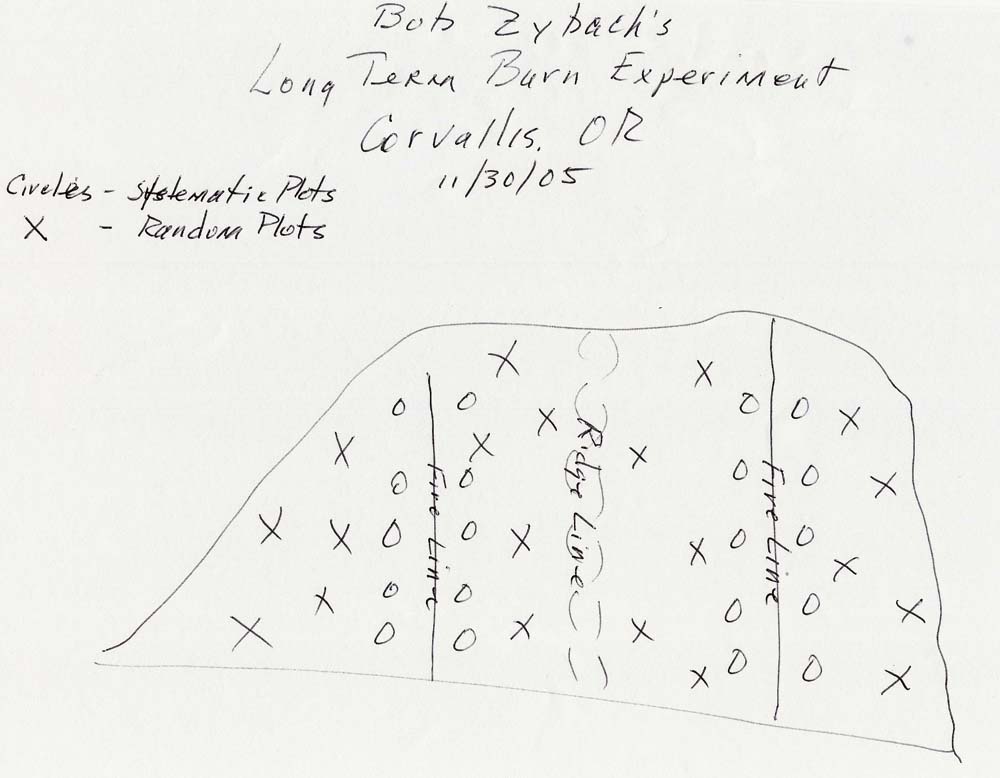
On page 2 I have sketched the experimental area as I remember the details.
There are 40 plots; 20 are systematically placed along the fire lines and 20 are randomly located in the other parts of the area. The middle area, with the ridgeline, is approximately twice as large as the two end areas.
Using the ideas from several texts on the analysis of attribute data, for you the presence or absence of a species, here is what I suggest:
For each species of interest you would determine presence or absence (P/A) in each plot the first year. This will be your baseline data against which you will compare data from subsequent years for each species.
With the 40 plots you will be able to compare P/A in the systematic vs. random plots, between east and west side of the ridgeline and elevation differences.
The statistic of choice is the chi square distribution. In general chi-square is used to determine whether an actual value is significantly different from expected values.
I have numbered the rows R for random and S for systematic from the bottom to the top of the sketch. The Rs are not in rows but are treated as so in the table.
| R1 | S1 | S2 | R2 | R3 | S3 | S4 | R4 |
| 0.0 | 1 | 0.0 | 1 | 0.0 | 1 | 1 | 0.0 |
| 1 | 0.0 | 0.0 | 1 | 0.0 | 0.0 | 0.0 | 1 |
| 1 | 0.0 | 1 | 0.0 | 1 | 0.0 | 1 | 0.0 |
| 0.0 | 1 | 1 | 0.0 | 1 | 1 | 1 | 1 |
| 0.0 | 1 | 0.0 | 1 | 0.0 | 1 | 0.0 | 0.0 |
| 2 | 3 | 2 | 3 | 2 | 3 | 3 | 2 |
| 5 | 5 | 5 | 5 | ||||
| 10 | 10 | ||||||
| 0.0 | 0.0 | 0.0 | 0.0 | 0.0 | 0.0 | 0.0 | 0.0 |
| 0.0 | 0.0 | 0.0 | 1 | 1 | 0.0 | 0.0 | 0.0 |
| 0.0 | 0.0 | 1 | 1 | 1 | 1 | 0.0 | 0.0 |
| 0.0 | 1 | 1 | 1 | 1 | 1 | 1 | 0.0 |
| 1 | 1 | 1 | 1 | 1 | 1 | 1 | 1 |
| 1 | 2 | 3 | 4 | 4 | 3 | 2 | 1 |
| 3 | 7 | 7 | 3 | ||||
| 10 | 10 | ||||||
The top table is designed to represent a random distribution of plants on a P/A basis. Chi square calculations would be:
X2 = (2-2.5)2/2.5 + (3-2.5)2/2.5 … for six more times. This is say that each column should have an average of 2.5 presences.
The general formula for X2 = the sum of the observed frequency – the expected frequency squared divided by the expected frequency for all eight columns. Doing the arithmetic, one gets a value of 0.2 for each of the eight columns for a total of 1.6. If one looks in a probability table for chi square you find that a value of 1.6 of about .30—highly likely to be due to chance.
Doing the second table in the same way one gets a chi square of 4.0, which had a probability of between 0.05 and 0.025. Such a distribution would be unlikely due to chance.
After you do your initial surveys for each species you will have expected values for each one. After the treatments you will see if the observed frequency has changed from what is was before the treatment.
You may, at a later time, want to look at other groupings of the plots. In whatever way you group them the calculation of chi-square would be carried out in a similar way.
Take a look at this, then we can talk about it and clear up any confusion that might exist. Thinking about this for your students is exciting. It will be hard evidence that before one goes collecting data that they know how the data are to be analyzed.
Best regards, Ben